A lot of people from engineering and non-engineering departments have trouble with the frequency domain. Many people can show you the frequency domain representation of a time domain signal, but not many can tell you what it means physically or visually. If the best teacher is experience, then no one will have a clue of what lies in the physical representation of the frequency domain. This is mainly because no one thinks in terms of frequency. If a signal is shown to you in the time domain (for example, a rectangular pulse) it is much easier to think of it as just a rectangular signal and not as anything else. This article will show you how to better understand the frequency domain representation of a signal with as little mathematics as possible, and also show you why it is more convenient in a lot of cases to use the frequency domain for signal analysis. For those not familiar with the frequency domain, this article will give a good introduction of what exactly the meaning of frequency domain is.

Time Domain

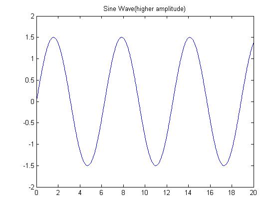
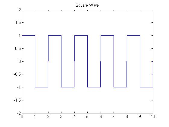
Most of the graphs you have seen are in the time domain. Any graph which plots time on one axis and amplitude on the other shows you the signal in the time-domain.

Believe it or not, each and every one of the signals shown above is actually made up of a number of sinusoidal signals, like this one:

Now, there are a number of properties we can change of this single sine signal, which forms the base of understanding how we derive the frequency domain.

Properties of a Sinusoidal Signal

The sine signal may look like a simple wave, but there are actually a lot of things we can modify.

Amplitude:  The amplitude is the measure of the height of the peaks of the signal. It is a measure of how intense the signal is. Higher the peaks of the signal, higher is the amplitude.

Frequency:Frequency is the number of times the wave repeats itself. In simpler terms, it is a measure of how many times the signal goes up-and-down about the zero point.

Phase:  the ‘phase’ of a sine signal shows how ‘late’ or how ‘early’ it is with respect to the starting point. Since a sine wave repeats itself(its periodic) so does the phase . It can vary from 0 to 359 degrees in angle and 360° is considered to be 0. For more advanced signals and calculations, phases beyond 360° are also used.

Assuming that the wave is moving from the right to the left of the page, we can compare the phases of the two signals shown.

Constructing the Frequency plot

Constructing the Frequency plot:

The construction of a frequency plot is best shown with an example. Let us consider a very common example of the fourier series of a rectangular wave of period 2s. It will look like this:

The Fourier series is:

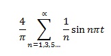
Now if we consider the first three terms of the series, we see that they are all sine waves, which are:

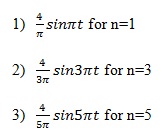Considering the three properties of a sine wave discussed earlier, we see that the amplitude and frequency change for each sine wave. If we plot the amplitude of each sine wave on the y axis and its corresponding frequency on the x axis, then we have the amplitude spectrum.

Similarly, if we plot the phase of each sine wave on the y axis and its corresponding frequency on the x axis, then we get the phase spectrum. In this case the phase of all the sine waves considered is 0 hence the phase spectrum will just be a straight line running on the x axis.

The amplitude and phase spectrum together completely describe any signal in terms of the sine waves that constitute it, and we call it the ‘frequency domain’

Signals which are non-periodic cannot be represented by a finite number of periodic signals. This is where we hear of the terms ‘frequency band’ and ‘bandwidth’. This means that the particular signal is made up of infinitely many sinusoidal waves within a particular range of frequencies called the ‘frequency band’. The difference between the upper most and the lowermost frequency of the band gives you the familiar term ‘bandwidth’

Why think in terms of frequency?

One might think it more convenient to think in terms of the time domain rather than the frequency domain. After all, it’s much easier to visualize time because we experience time every minute of our lives. Let us look at an example:

The above signal is called an amplitude modulated signal, and is commonly seen in radio communication. Now we cannot easily say anything meaningful about this signal other than that it’s a weirdly shaped sine signal. Now let us look at how the same signal is represented in the frequency domain.

That looks much simpler than the previous graph. We can now infer that the signal is made out of three sine signals (positive frequency). Furthermore, we can also see the amplitude of these signals and the frequency band they are a part of. This is especially important if we are to design filters to obtain the individual signals from the given signal.

Project Source Code

Project Source Code

###


%square wave
x=0:.1:20;
y=square(x,50);
plot(x,y);
title('Square Wave');
axis([0 20 -2 2]);
 
----------------
%sawtooth wave
x=0:20;
y=sawtooth(x);
plot(x,y);
title('Sawtooth Wave');
axis([0 20 -2 2]);
--------------------
%pulse wave
x=0:.1:20;
y=[zeros(1,50) ones(1,101) zeros(1,50)];
plot(x,y);
title('pulse');
axis([0 20 -2 2]);
---------------------
%higher and lower amplitude waves
x=0:.02:20;
y=1.5*sin(x);
plot(x,y);
title('Sine Wave(higher amplitude)');
axis([0 20 -2 2]);
 
x=0:.02:20;
y=.5*sin(x);
plot(x,y);
title('Sine Wave(lower amplitude)');
axis([0 20 -2 2]);
-------------------
%higher and lower frequency waves
x=0:.02:20;
y=sin(4*x);
plot(x,y);
title('Sine Wave(high frequency)');
axis([0 20 -2 2]);
x=0:.02:20;
y=sin(.5*x);
plot(x,y);
title('Sine Wave(low frequency)');
axis([0 20 -2 2]);
----------------------------
%sine waves of different phases
x=0:.02:20;
y=sin(x+.2);
plot(x,y);
title('Sine Wave(delayed)');
axis([0 20 -2 2]);
 
x=0:.02:20;
y=sin(x);
plot(x,y);
title('Sine Wave(undelayed)');
axis([0 20 -2 2]);
--------------------------
%square wave of 2s period
x=0:.01:10;
y=square(pi*x,50);
plot(x,y);
title('Square Wave');
axis([0 10 -2 2]);
--------------------------
%amplitude spectrum
x=[1 3 5 7 9 11 13 15 17 19];
y=4./(pi*x);
stem(x,y);
title('Amplitude spectrum');
axis([0 20 -.5 1.5 ]);
-------------------------
%amplitude modulated wae
x=0:.01:10;
y=sin(10*x).*sin(x);
plot(x,y);
title('AM Wave');
axis([0 10 -2 2]);
------------------------
%frequency representation of am wave
x=0:12;
y=[0 0 0 0 0 0 0 0