Digital Signal Processing Tutorial: Discrete Time Systems and their Classification

In the previous tutorial we learnt about the Sampling Process, Discrete-time signals, their classification and also had an idea about transformation of discrete-time signals. These topics are the most basic and important entities of DSP. Now we will be studying about the systems which process these signals to give the desired form of output signals.

What we are going to learn in this tutorial:-

Discrete-time Systems

Classification of Discrete-time Systems

Discrete-time systems

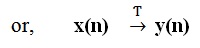
Discrete-time systems, “A set of connected parts or models which takes discrete-time signals as input, known as excitation, processes it under certain set of rules and algorithms to have a desired output of another discrete-time signal, known as response”. In general, if a there is excitation x(n) and the response of the system is y(n), the we express the system as,

y(n) = T [x(n)]

DSP

Where, T is the general rule or algorithm which is implemented on x(n) or the excitation to get the response y(n). For example, a few systems are represented as,

y(n) = -2x(n)

or, y(n) = x(n-1) + x(n) + x(n+1)

Block Diagram representation of Discrete-time systems

Digital Systems are represented with blocks of different elements or entities connected with arrows which also fulfills the purpose of showing the direction of signal flow,

Block Diagram of Discrete Time System

Fig. 1: Block Diagram of Discrete Time System

Some common elements of Discrete-time systems are:-

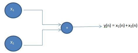
· Adder: It performs the addition or summation of two signals or excitation to have a response. An adder is represented as,

Block Diagram of Adder

Fig. 2: Block Diagram of Adder

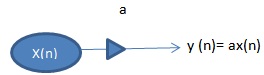
· Constant Multiplier: This entity multiplies the signal with a constant integer or fraction. And is represented as, in this example the signal x(n) is multiplied with a constant “a” to have the response of the system as y(n).

Block Diagram of Constant Multiplier

Fig. 2: Block Diagram of Constant Multiplier

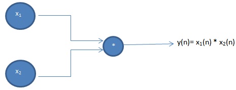
·Signal Multiplier: This element multiplies two signals to obtain one.

Block Diagram of Signal Multiplier

Fig. 3: Block Diagram of Signal Multiplier

·Unit-delay element: This element delays the signal by one sample i.e. the response of the system is the excitation of previous sample. This can element is said to have a memory which stores the excitation at time n-1 and recalls this excitation at the time n form the memory. This element is represented as,

Block Diagram of Unit Delay Element

Fig. 4: Block Diagram of Unit Delay Element

·Unit-advance element: This element advances the signal by one sample i.e. the response of the current excitation is the excitation of future sample. Although, as we can see this element is not physically realizable unless the response and the excitation are already in stored or recorded form.

Block Diagram of Unit Advance Element

Fig. 5: Block Diagram of Unit Advance Element

Now that we have understood the basic elements of the Discrete-time systems we can now represent any discrete-time system with the help of block diagram. For example,

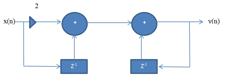
y(n) = y(n-1) + x (n-1) + 2x(n)

Block Diagram of Example Discrete Time System

Fig. 6: Block Diagram of Example Discrete Time System

The above system is an example of Discrete-time system involving the unit delay of current excitation and also one unit delay of the current response of the system. This system can be said to be a Dynamic System, but as we don’t know anything about the classification of a discrete-time system, we are going to learn about the classification of systems to have a better understanding of discrete-time systems.

Classification of Discrete-time Systems

Classification of Discrete-time System

Discrete-time systems are classified on different principles to have a better idea about a particular system, their behavior and ultimately to study the response of the system.

Relaxed system: If y(n_o-1) is the initial condition of a system with response y(n) and y(n_o-1)=0 , then the system is said to be initially relaxed i.e. if the system has no excitation prior to n_o .

Static and Dynamic systems: A system is said to be a Static discrete-time system if the response of the system depends at most on the current or present excitation and not on the past or future excitation. If there is any other scenario then the system is said to be a Dynamic discrete–time system. The static systems are also said to be memory-less systems and on the other hand dynamic systems have either finite or infinite memory depending on the nature of the system. Examples below will clear any arising doubts regarding static and dynamic systems.

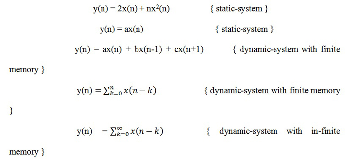
Image showing examples of static and dynamic systems

Fig. 7: Image showing Examples of Static and Dynamic Systems

The last example is the case of in-finite memory and the others are specified about their type depending on their characteristics.

Time-variant and Time-invariant system: A discrete-time system is said to be time invariant if the input-output characteristics do not change with time, i.e. if the excitation is delayed by k units then the response of the system is also delayed by k units. Let there be a system,

x(n) —->^T y(n) V x(n)

Then the relaxed system T is time-invariant if and only if,

x(n-k) —->^T y(n-k) V x(n) and k.

Otherwise, the system is said to be time-variant system if it does not follows the above specified set of rules. For example,

y(n) = ax(n) { time-invariant }

y(n) = x(n) + x(n-3) { time-invariant }

y(n) = nx(n) { time-variant }

Note:- In order to check whether the system is time-invariant or time-variant the system must satisfy the “T[x(n-k)]=y(n-k)” condition, i.e. first delay the excitation by k units, then replace n with (n-k) in the response and then equate L.H.S. and R.H.S. if they are equal then the system is time invariant otherwise not. For example in the last system above,

L.H.S. = T[x(n-k)] =nx(n-k) {not (n-k)x(n-k) which is a general misconfusion}

R.H.S. = y(n-k)= (n-k) x(n-k)

So, the L.H.S. and R.H.S. are not equal hence the system is time-varient.

Note:- What about Folder, is it a time-variant or time-invariant system, let’s see,

y(n) = x(-n)

L.H.S. = y(n-k) = x[-(n-k)]=x(-n+k)

R.H.S. = T[x(n-k)] = x(-n-k)

Thus, R.H.S. is not equal to L.H.S. so the system is time-variant.

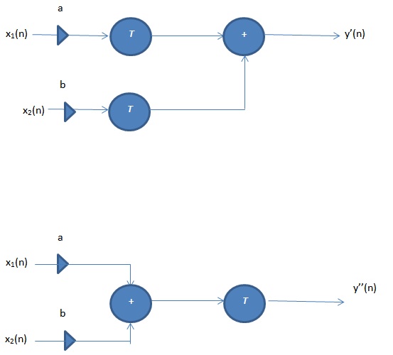
Linear and non-Linear systems: A system is said to be a linear system if it follows the superposition principle i.e. the sum of responses (output) of weighted individual excitations (input) is equal to the response of sum of the weighted excitations. Pay attention to the above specified rule, according to the rule the following condition must be fulfilled by the system in order to be classified as a Linear system,

If, y₁(n) = T[ ax₁(n) ]

y₂(n) = T[ bx₂(n) ]

and, y(n) = T[ax₁(n) + bx₂(n)]

Then, the system is said to be linear if ,

T[ ax₁(n) + bx₂(n)] = T[ ax₁(n) ] + T[ bx₂(n) ]

Block Diagram of Linear and Non-Linear Systems

Fig. 8: Block Diagram of Linear and Non-Linear Systems

So, iff y’(n) = y’’(n) then the system is said to be linear. I the system does not fulfills this property then the system is a non-Linear system. For example,

y(n) = x (n²) { linear }

y(n) = Ax(n) + B {non – linear }

y(n) = nx(n) { linear }

The explanation of the above specified examples is left as an exercise for the reader.

Causal and non-Causal systems: A discrete-time system is said to be a causal system if the response or the output of the system at any time depends only on the present or past excitation or input and not on the future inputs. If the system T follows the following relation then the system is said to be causal otherwise it is a non-causal system.

y(n) = F [x(n), x(n-1), x(n-2),…….]

Where F[] is any arbitrary function. A non-causal system has its response dependent on future inputs also which is not physically realizable in a real-time system but can be realized in a recorded system. For example,

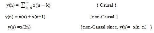
Image showing casual and non-casual systems

Fig. 9: Image Showing Casual and Non-Casual Systems

Stable and Unstable systems: A system is said to be stable if the bounded input produces a bounded output i.e. the system is BIBO stable. If,

Stable and Unstable Systems

Then the system is said to be bounded system and if this is not the case then the system is unbounded or unstable.

This tutorial gave idea about the classification of systems as it is necessary to know some basic properties of the system for easy analysis. In the nest tutorial we will be studying about LTI(Linear and Time Invariant) systems and their properties and will also, if the time permits, see z-transformation which is done for the analysis of the systems and is analogous to Fourier transform in analog communications.